In financial mathematics and stochastic optimization, the concept of risk measure is used to quantify the risk involved in a random outcome or risk position. Many risk measures have hitherto been proposed, each having certain characteristics. The entropic value at risk (EVaR) is a coherent risk measure introduced by Ahmadi-Javid,[1][2] which is an upper bound for the value at risk (VaR) and the conditional value at risk (CVaR), obtained from the Chernoff inequality. The EVaR can also be represented by using the concept of relative entropy. Because of its connection with the VaR and the relative entropy, this risk measure is called "entropic value at risk". The EVaR was developed to tackle some computational inefficiencies[clarification needed] of the CVaR. Getting inspiration from the dual representation of the EVaR, Ahmadi-Javid[1][2] developed a wide class of coherent risk measures, called g-entropic risk measures. Both the CVaR and the EVaR are members of this class.
Definition
Let be a probability space with a set of all simple events, a -algebra of subsets of and a probability measure on . Let be a random variable and be the set of all Borel measurable functions whose moment-generating function exists for all . The entropic value at risk (EVaR) of with confidence level is defined as follows:
(1)
In finance, the random variable in the above equation, is used to model the losses of a portfolio.
which shows the relationship between the EVaR and the Chernoff inequality. It is worth noting that is the entropic risk measure or exponential premium, which is a concept used in finance and insurance, respectively.
Let be the set of all Borel measurable functions whose moment-generating function exists for all . The dual representation (or robust representation) of the EVaR is as follows:
(3)
where and is a set of probability measures on with . Note that
is the relative entropy of with respect to also called the Kullback–Leibler divergence. The dual representation of the EVaR discloses the reason behind its naming.
Properties
The EVaR is a coherent risk measure.
The moment-generating function can be represented by the EVaR: for all and
(4)
For , for all if and only if for all .
The entropic risk measure with parameter can be represented by means of the EVaR: for all and
(5)
The EVaR with confidence level is the tightest possible upper bound that can be obtained from the Chernoff inequality for the VaR and the CVaR with confidence level ;
(6)
The following inequality holds for the EVaR:
(7)
where is the expected value of and is the essential supremum of , i.e., . So do hold and .
Examples
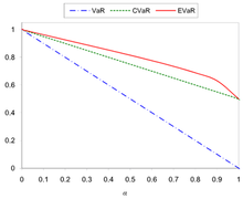
Comparing the VaR, CVaR and EVaR for the standard normal distributionComparing the VaR, CVaR and EVaR for the uniform distribution over the interval (0,1)
For
(8)
For
(9)
Figures 1 and 2 show the comparing of the VaR, CVaR and EVaR for and .
Optimization
Let be a risk measure. Consider the optimization problem
(10)
where is an -dimensional real decision vector, is an -dimensional real random vector with a known probability distribution and the function is a Borel measurable function for all values If then the optimization problem (10) turns into:
(11)
Let be the support of the random vector If is convex for all , then the objective function of the problem (11) is also convex. If has the form
which is computationally tractable. But for this case, if one uses the CVaR in problem (10), then the resulting problem becomes as follows:
(14)
It can be shown that by increasing the dimension of , problem (14) is computationally intractable even for simple cases. For example, assume that are independent discrete random variables that take distinct values. For fixed values of and the complexity of computing the objective function given in problem (13) is of order while the computing time for the objective function of problem (14) is of order . For illustration, assume that and the summation of two numbers takes seconds. For computing the objective function of problem (14) one needs about years, whereas the evaluation of objective function of problem (13) takes about seconds. This shows that formulation with the EVaR outperforms the formulation with the CVaR (see [2] for more details).
Generalization (g-entropic risk measures)
Drawing inspiration from the dual representation of the EVaR given in (3), one can define a wide class of information-theoretic coherent risk measures, which are introduced in.[1][2] Let be a convex proper function with and be a non-negative number. The -entropic risk measure with divergence level is defined as
(15)
where in which is the generalized relative entropy of with respect to . A primal representation of the class of -entropic risk measures can be obtained as follows:
(16)
where is the conjugate of . By considering
(17)
with and , the EVaR formula can be deduced. The CVaR is also a -entropic risk measure, which can be obtained from (16) by setting
For more results on -entropic risk measures see.[4]
Disciplined Convex Programming Framework
The disciplined convex programming framework of sample EVaR was proposed by Cajas[5] and has the following form:
(19)
where , and are variables; is an exponential cone;[6] and is the number of observations. If we define as the vector of weights for assets, the matrix of returns and the mean vector of assets, we can posed the minimization of the expected EVaR given a level of expected portfolio return as follows.
(20)
Applying the disciplined convex programming framework of EVaR to uncompounded cumulative returns distribution, Cajas[5] proposed the entropic drawdown at risk(EDaR) optimization problem. We can posed the minimization of the expected EDaR given a level of expected return as follows:
(21)
where is a variable that represent the uncompounded cumulative returns of portfolio and is the matrix of uncompounded cumulative returns of assets.
For other problems like risk parity, maximization of return/risk ratio or constraints on maximum risk levels for EVaR and EDaR, you can see [5] for more details.
The advantage of model EVaR and EDaR using a disciplined convex programming framework, is that we can use softwares like CVXPY [7] or MOSEK[8] to model this portfolio optimization problems. EVaR and EDaR are implemented in the python package Riskfolio-Lib.[9]
^ abcdAhmadi-Javid, Amir (2011). "An information-theoretic approach to constructing coherent risk measures". 2011 IEEE International Symposium on Information Theory Proceedings. St. Petersburg, Russia: Proceedings of IEEE International Symposium on Information Theory. pp. 2125–2127. doi:10.1109/ISIT.2011.6033932. ISBN 978-1-4577-0596-0. S2CID 8720196.
^ abcdAhmadi-Javid, Amir (2012). "Entropic value-at-risk: A new coherent risk measure". Journal of Optimization Theory and Applications. 155 (3): 1105–1123. doi:10.1007/s10957-011-9968-2. S2CID 46150553.
^Ahmadi-Javid, Amir (2012). "Addendum to: Entropic Value-at-Risk: A New Coherent Risk Measure". Journal of Optimization Theory and Applications. 155 (3): 1124–1128. doi:10.1007/s10957-012-0014-9. S2CID 39386464.
^Breuer, Thomas; Csiszar, Imre (2013). "Measuring Distribution Model Risk". arXiv:1301.4832v1 [q-fin.RM].


![{\displaystyle \alpha \in ]0,1]}](https://wikimedia.org/api/rest_v1/media/math/render/svg/d807843c397d6655a0415841bfd2d942aaa9f738)


![{\displaystyle \min _{{\boldsymbol {w}}\in {\boldsymbol {W}},t\in \mathbb {R} }\left\lbrace t+{\frac {1}{\alpha }}{\text{E}}\left[g_{0}({\boldsymbol {w}})+\sum _{i=1}^{m}g_{i}({\boldsymbol {w}})\psi _{i}-t\right]_{+}\right\rbrace .}](https://wikimedia.org/api/rest_v1/media/math/render/svg/8fd60d85fb67797f3d44f5741f97314be2072986)


![{\displaystyle {\text{ER}}_{g,\beta }(X)=\inf _{t>0,\mu \in \mathbb {R} }\left\lbrace t\left[\mu +{\text{E}}_{P}\left(g^{*}\left({\frac {X}{t}}-\mu +\beta \right)\right)\right]\right\rbrace }](https://wikimedia.org/api/rest_v1/media/math/render/svg/03980f4d09c2a5a913ca0a64866c3a747d851fd5)


